CMInject User guide ¶

Welcome to the User guide for CMInject! CMInject is a Python3 framework for defining and running nanoparticle trajectory simulations.

Contents

CMInject User guide

Prerequisites ¶

On some systems, in particular for Python version 3.6, it may be necessary to install the HDF5 libraries before attempting to install CMInject.

Installation ¶

We strongly recommend the use of a virtual environment (venv 2) for CMInject. If you cannot use virtual environments for whatever reason, simply skip the first two steps.

Create a virtual environment with venv 2 in a directory of your choice:
```
python3 -m venv /some/dir
```

Activate the virtual environment (run the applicable Command):

Platform	Shell	Command
POSIX	bash/zsh	source /some/dir/bin/activate
	fish	. /some/dir/bin/activate.fish
	fish	. /some/dir/bin/activate.fish
	csh/tcsh	source /some/dir/bin/activate.csh
	csh/tcsh	source /some/dir/bin/activate.csh
	PowerShell Core	source /some/dir/bin/Activate.ps1
	PowerShell Core	source /some/dir/bin/Activate.ps1
Windows	cmd.exe	some\dir\Scripts\activate.bat
Windows	PowerShell	some\dir\Scripts\Activate.ps1

Install Cython and numpy (required for installation):
```
pip install Cython numpy
```
Install CMInject:

Switch (cd) to the directory where you downloaded/cloned CMInject. Then:
- If you just want to use CMInject:
```
python setup.py install
```
- If you also plan on developing CMInject (see setup.py develop 1):
```
python setup.py develop
```

Running CMInject ¶

A toy simulation with ExampleSetup ¶

A very simple simulation can be run by using the cminject program, running the setup cminject.setups.example.ExampleSetup:

cminject \
  -s cminject.setups.example.ExampleSetup   `# Use ExampleSetup`\
  -f examples/2d_example_field.h5           `# Use the 2D example field`\
  -n 100                                    `# Simulate 100 particles`\
  -o examples/example_output.h5             `# Write the results to example_output.h5`\
  -T                                        `# Track and store trajectories`

The example field is provided in the examples/ subdirectory of CMInject. You can then try out the following:

Adding the parameter --pos G[0,1e-4] 0, which sets the x/z position distributions to

x: A normal (Gaussian) distribution with µ=0.0, σ=10^-4 (narrower than default σ=10^-3)

z: Constant 0

Adding the parameter --loglevel info to get details about the start and end of each particle’s simulation, e.g., the ending time and reason.

Adding the parameter -h to get informative help text about all available parameters; see also Getting help.

Visualizing the output data with cminject_visualize -T examples/example_output.h5; see also cminject_visualize.

The simulation using ExampleSetup is straightforward to understand, but not very flexible. For example, the starting velocities and detector positions are not exposed as parameters, and so are fixed.

A more realistic, but more complex call of cminject could be

cminject -n 100          `# Run the simulation for 100 particles.`\
  -D 3                   `# Use a spatial dimensionality of 3.`\
  -f flowfield.h5        `# Use the flow field file flowfield.h5. Must be a 3D flow field\
                          # since we specified -D 3.`\
  -rho 1050 -r 50e-9     `# Simulate particles with a density of 1050kg/m^3\
                          # and a radius of 50nm`\
  -p G[0,1e-3] 0 0       `# Randomly generate initial particle positions, the first dimension\
                          # (x) being normally (gaussian) distributed with mu = 0m and\
                          # sigma = 1mm, and the others (y, z) being fixed at 0m.`\
  -v G[0,1] 0 -10.0      `# Randomly generate initial particle velocities, the first dimension\
                          # being normally (gaussian) distributed with mu = 0m/s and\
                          # sigma = 1m/s, the second (y) fixed at 0m/s, and the third (z)\
                          # fixed at -10.0m/s.`\
  -d 0 -0.01             `# Insert virtual detectors at 0m and -1cm`\
  -T                     `# Track and store trajectories`\
  -B                     `# Enable Brownian motion`\
  -o output.h5           `# Write results to output.h5`

We do not use ExampleSetup here. Since the setup is not provided explicitly, the default setup is used (see cminject.setups.one_flow_field.OneFlowFieldSetup). All provided setups are listed in cminject.setups package.

Note

cminject, for now, only accepts HDF5 files as flow fields (i.e., the -f argument). See cminject_txt-to-hdf5 for information on how to convert TXT files that define a grid field to such HDF5 files.

Getting help ¶

If you want to find out all available parameters, you can add the -h option to any call of the cminject program. If you’ve picked a specific setup with the -s option, the parameters available for this setup will also be listed and explained.

Further steps ¶

The output files of both simulations described above can be viewed with cminject_visualize. They can also be further analyzed, e.g., directly with cminject_analyze-asymmetry, or by manually working with the stored data. These tools are described in List of utility programs.

Result data can be retrieved from the cminject.result_storages.hdf5.HDF5ResultStorage class, which can benstantiated with the filename of the result file, and offers a straightforward interface to retrieve each piece of stored result data.

Result data access ¶

CMInject simulations write HDF5 result files to disk, using the class cminject.result_storages.HDF5ResultStorage. You can read back and use this data through a convenient Python interface, or by using HDF5 itself as a low-level interface, from any other software that handles HDF5 files.

Convenient interface ¶

The easiest way to retrieve and use this result data for your further analyses is to use that same class cminject.result_storages.HDF5ResultStorage, since it offers methods for data retrieval like cminject.result_storages.HDF5ResultStorage.get_detectors() or cminject.result_storages.HDF5ResultStorage.get_trajectories().

As an example, we can retrieve the detectors (as a dictionary) by calling get_detectors() on a HDF5ResultStorage instance constructed with our result file’s name, output.h5:

from cminject.result_storages import HDF5ResultStorage
with HDF5ResultStorage('output.h5') as rs:
  detectors = rs.get_detectors()
  # ... do something with detectors, e.g., plot the x distribution of one detector at z=0:
  plt.figure(); plt.hist(detectors['SimpleZ@0']['position'][:, 0])

See the class documentation here: cminject.result_storages.HDF5ResultStorage, for a full list of available data retrieval methods. Their names all start with get_.

Low-level interface ¶

The low-level interface is just the HDF5 file format itself, used with a specific structure for our result outputs. We have documented this output structure in the docstring of the cminject.result_storages.HDF5ResultStorage class.

List of utility programs ¶

There are other programs to prepare input data to, and process, analyze and visualize output data from cminject. This section gives a list of all these programs contained in CMInject and describes each of them.

cminject_txt-to-hdf5 ¶

cminject_txt-to-hdf5 was written to convert TXT files describing a field as a regular grid, like flow field files, to HDF5 files. For example, the COMSOL Multiphysics software writes out such TXT files. The reason this is useful is that large TXT files are very slow to read in in comparison to HDF5 files.

To convert a file, run cminject_txt-to-hdf5 -i <infile.txt> -o <outfile.h5> -d <dimensions>. For convenience, you can store arbitrary attributes on the converted .h5 file that can be read by CMInject’s code, so you don’t need to pass them when running the program. A typical set of such attributes to store is -fG and -ft, which store the gas type and temperature the field was defined with.

Warning

If the TXT file you are converting was generated for axisymmetric data, it might only contain entries for positive coordinates (e.g., the r in r/z coordinates). Since cminject does not know about this fact, particles might well cross into “negative r” and be considered ‘lost’ since they are, coordinate-wise, outside of the field. In this case, please use the -m option for cminject_txt-to-hdf5, which mirrors the available data around the axis of symmetry and thus allows simulations to work as expected.

cminject_visualize ¶

cminject_visualize visualizes result files. After you’ve run a simulation with cminject [...] -o resultfile.h5, you can visualize this result file by running cminject_visualize. There are currently two options for visualizing results available:

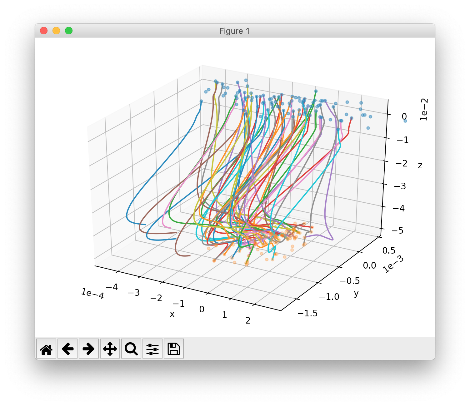
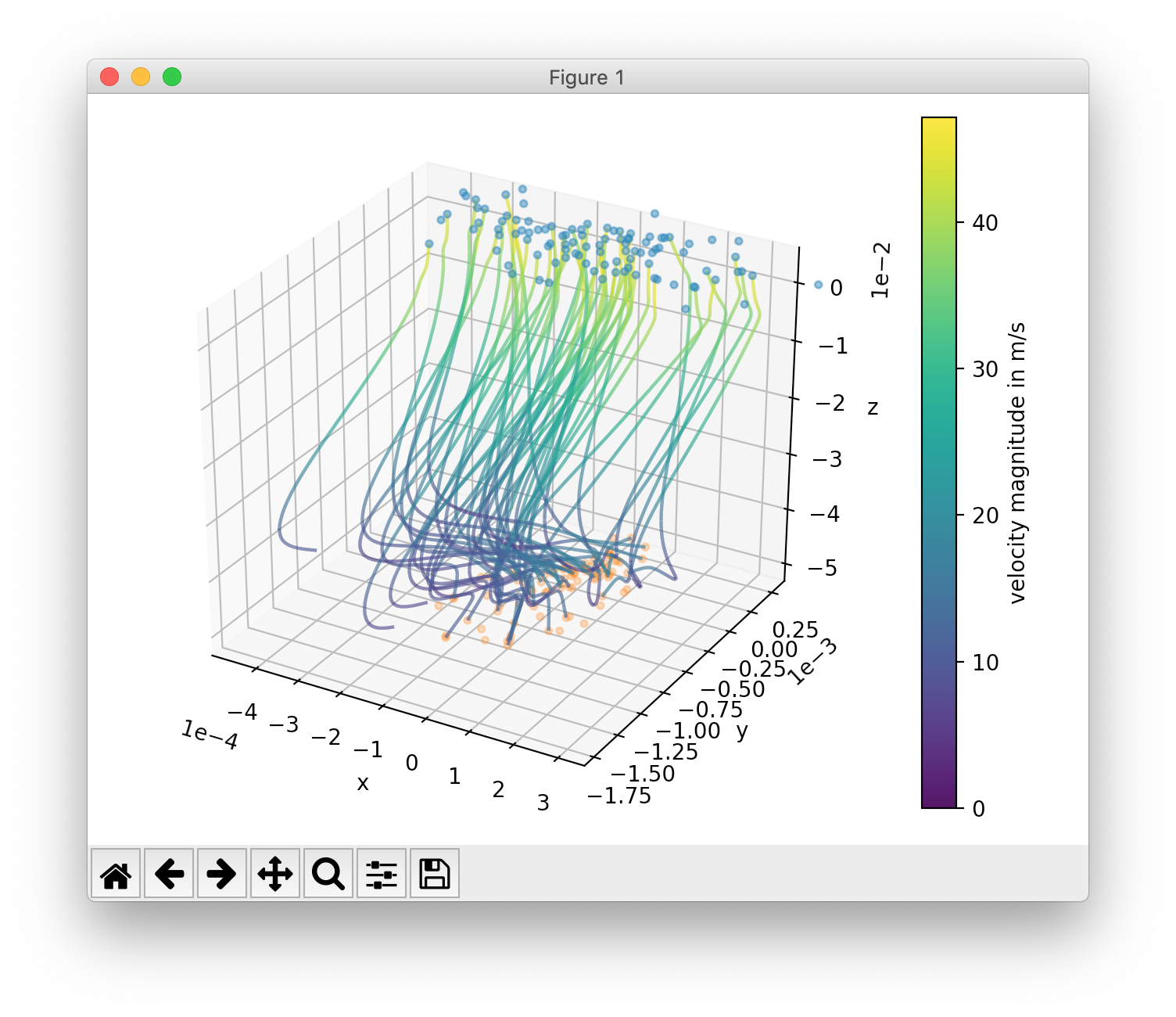
A trajectory visualization, which can be shown with -T and optionally configured through other parameters starting with -T. It shows both trajectories as curves, and detectors as scatter plots:

cminject_visualize
  resultfile.h5        # For resultfile.h5...
  -T                   # ...show trajectory plots...
  -Tn 30               # ...of 30 randomly sampled particles,
  -Tc                  # using color coding for velocities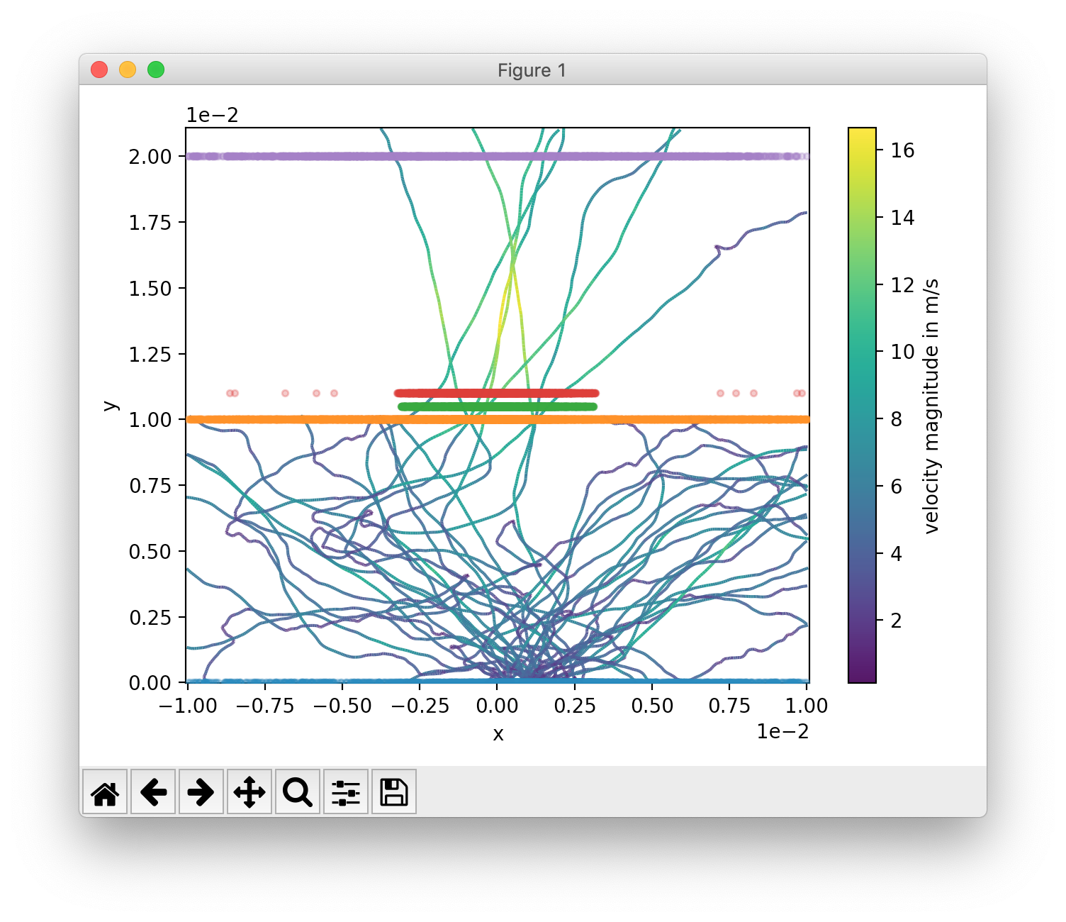

A detector histogram visualization (1D or 2D), which can be shown with -H x,y [x,y ...]:

# Show histograms for all stored detectors in resultfile.h5,
# for a collection of dimension pairs to be shown as histograms together.
# When one dimension has a constant value (e.g. z), a 1D histogram
# will be shown, otherwise a 2D histogram will be shown.
cminject_visualize resultfile.h5 -H x,y  x,z  y,z  x,vx  y,vy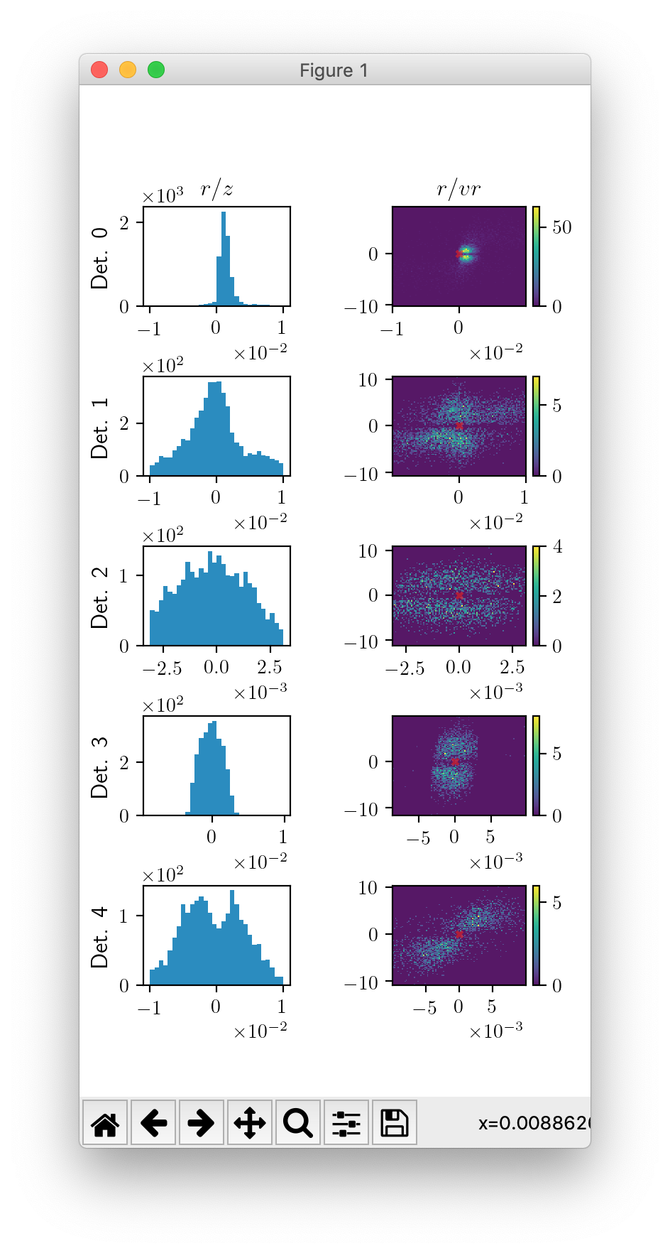

cminject_analyze-asymmetry ¶

cminject_analyze-asymmetry prints out information about the asymmetry of a 2D distribution at each stored detector. The output format can either be nicely formatted text to be human-readable, or CSV with the --csv parameter, for further data processing. An example call:

cminject_analyze-asymmetry
   resultfile.h5   # Print the analysis results for resultfile.h5,
   --x 0 --y 1     # using the stored property at index 0 as the first
                   # dimension and the one at index 1 as the second.

which prints, for example, the following output:

-------------------- Detector 0 --------------------
α: 0.199
e₀ = 6.473e-06       e₁ = 9.693e-06
θ₀ = -0.451π         θ₁ = -0.951π
μx = -1.658e-05      μy = -3.031e-05

-------------------- Detector 1 --------------------
α: 0.934
e₀ = 3.877e-07       e₁ = 1.132e-05
θ₀ = -0.523π         θ₁ = 0.977π
μx = -2.867e-05      μy = -3.195e-04

This output can instead be printed as machine-readable CSV by passing the --csv flag parameter.

References ¶

1: https://setuptools.readthedocs.io/en/latest/setuptools.html#develop-deploy-the-project-source-in-development-mode
2(1,2): https://docs.python.org/3/library/venv.html